 中文版本
中文版本

- Home
- » Linking Theory to Reality
- » Evolutionary approaches
Evolutionary Approaches
Evolutionary approaches are based on the idea that a full understanding of modern systems can only come through observing how they came into being. This means taking a longer time perspective than many conventional studies, drawing on all kinds of data and information sources so that we can anlayse the trends, interactions and overall system dynamics that produced the modern state. The approach rests firmly on the idea that complex systems emerge or evolve through a combination of external drivers and internal self-organization with nonlinear responses that are not given to simple cause-and-effect explanations. There are a number of elements within the approach, including:
- Changing boundary conditions – the ‘natural’ background of controlling or constraining conditions change slowly and often determine the resilience of the whole system; e.g. imperceptibily slow rates of soil loss may only become important to crop production when the cumulative losses reach a certain threshold level.
- Legacies and contingencies - periodic perturbations affect future system development through lagged effects; e.g. artificial drainage may dry surface soils that affect the ability of trees to withstand windthrow - but only decades into the future when they are mature.
- Path dependency - the trajectory of a system where change is driven and self-reinforced by feedback mechanisms, giving rise to 'locked-in' behaviour leading to 'traps' e.g; intensive agriculture that is dependent on irrigation, pesticides and fertilizers even as natural soil fertility and local groundwater reserves decline is said to be 'locked-in' towards a 'rigidity trap' - where returning to traditonal methods is no longer an option but where there are few other option to just carrying on in the same way. At the other extreme, systems that are poorly connected and lacking capital move towards 'poverty traps' where the system can stagnate.
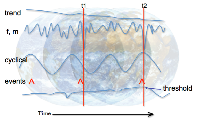
Figure: A Perfect Storm conceptual model of social-ecological change through the interaction of multiple factors. The change in the dependent variable is the combined result of several types of other interacting variables represented as long-term trends, irregular (frequency and magnitude) and periodic variables, as well as discrete events (A). In this example, the long-term trend that determines resilience has decreased sufficiently at t2 to make the system sensitive to a combination of other variable states (a minimum in the irregular variable, a maximum in the periodic variable, and the occurrence of an event A) and cause the dpendnet variable to collapse across a threshold. In contrast, similar conditions in the variables existed at t1 but the resilience was much higher, which in combination with the other independent variables did not result in a change in the dependent variable. A number of real world examples may be mapped onto this model, for example: major fires in California occur where long term, irregular, periodic and event signals correspond to the frequency of small fires, wind strength, seasonal climate and ignition events respectively; or the global stock market crisis where long term, irregular, periodic and event signals correspond to long term growth of sub-prime debt, commodity prices, seasonal housing market, and the failure of individual banks respectively (Dearing et al. 2012)